

In the world of data analytics, information is mined from various sources and gathered into meticulous piles to be organized, categorized, and synthesized into digestible formats for target audiences. Industrial Hygiene (IH) investigations are themselves a goldmine of raw data waiting to be digested. Many workplaces have years of past IH exposure monitoring data that can be used to make informed exposure assessment decisions, provided that statistical tools are utilized properly.
Many statistical analysis tools with training are available free of charge and readily accessible through industry groups such as the American Industrial Hygiene Association (AIHA). These tools utilize Bayesian statistical techniques to analyze trends in exposure monitoring data. Using this approach, exposure categories are assigned to the sample set based on the exposure results for each relevant Similar Exposure Group (SEG) using a defined decision statistic (e.g., the 95th percentile). This enables the Industrial Hygienist to determine the probability that the true 95th percentile of the exposure results would fall within one of the AIHA Exposure Rating Categories, which range from 0 (<1% of the Occupational Exposure Limit) to 4 (>100% of the OEL), where 0 represents a negligible exposure, and 4 represents a poorly controlled exposure. A confidence rating is also assigned to these results.
Looking at industrial hygiene data this way can tell us several things in a short time. By looking at the distribution, we can assess whether the chosen similar exposure groups (SEGs) were properly selected. We can tell whether the sampling rates are at the correct frequency and whether the sample sizes are adequate.
While Bayesian tools are great for statistical analysis, there are ways to take the data a step further. This is also true for any additional information that may be paired with quantitative results. Risk rankings, qualitative analysis, prevention through design, and audit findings, to name a few. The numeric output of any of these assessments can be placed into a visual data analytics tool to help drive decision-making and impact stakeholders.
It is important to ensure that your data is sound and your metrics are consistent across multiple collection events. The adage “garbage in equals garbage out” applies here and comes up very often in topical conversations. If establishing a new program, align on terms, units of measurement, and other similar parameters at the start. For seasoned programs, it is not too late to create a reference or dictionary. Once you have alignment, you can establish connections to form a total picture of true exposure risks and drive informed decision-making.
Modeling asbestos exposure data utilizing the Expo Stats Tool 1: Estimation of parameters of the lognormal distribution and comparison to an occupational exposure limit (OEL) can give a clearer picture as to the exposure risk for each of the following SEGs:
- SEG 1 – Gross removal of friable asbestos TSI from a pipe within a containment utilizing wet methods.
- SEG 2 – Performing fine cleaning following gross removal of asbestos TSI.
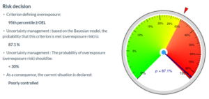
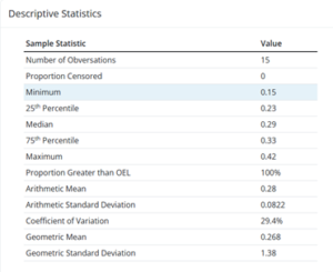
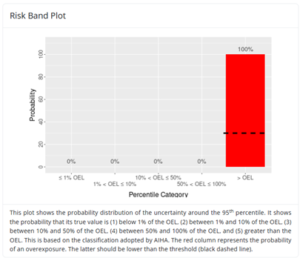
For this example, we will use mock personal air sampling results generated with industry knowledge and assume the data were collected over three separate projects, using the same five employees for gross removal and five employees for fine cleaning. Each SEG will have fifteen (15) data points presented as an 8-hour time-weighted average (TWA), and we will compare it to the Occupational Health and Safety Administration (OSHA) Permissible Exposure Limit (PEL) of 0.1 f/cc. The samples will have theoretically been analyzed via NIOSH Method 7400 phase contrast microscopy (PCM). Below are the statistics for each data set, presented numerically and graphically on the Risk Band Plot.
SEG 1
SEG 2
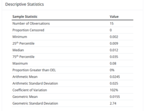
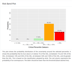
Using this data, we can better predict the likelihood of personal exposure to airborne asbestos fibers during these two specific work activities. This, in turn, helps determine the proper level of personal protective equipment (PPE), as well as other risk-reduction strategies such as engineering controls that may be used during abatement efforts. We can see from our specific examples that gross removal presents the highest risk of exposure above the PEL, and while fine cleaning following the gross removal presents a lower risk, it still has the potential to exceed the PEL. If we took this a step further and used data from an abatement project where wet methods were not utilized, we could really dig into just how statistically effective those methods are at reducing the exposure risk to airborne fibers.
Our example includes two very different results for the coefficient of variation showing the spread of our data. Results for SEG 1 have a smaller variation than SEG 2, which shows that the work practices in SEG 1 resulted in more consistent results. For our purposes, this may mean that SEG 2 includes additional sub-SEGs, such as workers performing scrubbing and HEPA vacuuming, while others are only removing waste bags, or perhaps the engineering practices were very different from job to job. It is easy to see from this example how having a smaller data set or adding SEGs with dissimilar work practices could easily skew our results and lead to an incorrect analysis of the risk. It is crucial that data sets, combined with a proper understanding of the SEGs, be utilized to continuously improve work practices.
References:
- American Industrial Hygiene Association. (n.d.). AIHA exposure risk assessment & management tools. AIHA. Retrieved July 22, 2026, from https://www.aiha.org/public-resources/healthierworkplaces/workplacehazards/apps-and-tools-resource-center/aiha-risk-assessment-tools
- Lavoué, J., Joseph, L., Knott, P., Davies, H., Labrèche, F., Clerc, F., Mater, G., & Kirkham, T. (2019). Expostats: A Bayesian toolkit to aid the interpretation of occupational exposure measurements. Annals of Work Exposures and Health, 63(3), 267–279. https://doi.org/10.1093/annweh/wxy100
- Université de Montréal. (n.d.). Expostats tools. Retrieved July 22, 2026, from https://expostats.ca/site/en/tools.html
- United States Environmental Protection Agency. (n.d.). Health and Environmental Research Online (HERO): Reference 3102271. Retrieved July 22, 2026, from https://hero.epa.gov/reference/3102271/
- Groth, C. P., Banerjee, S., Ramachandran, G., Stewart, P. A., Stenzel, M. R., & Virji, M. A. (2022). Quantifying worker exposures using Bayesian statistical methods in industrial hygiene. In Wiley StatsRef: Statistics Reference Online. John Wiley & Sons. https://doi.org/10.1002/9781118445112.stat08376
- Lange, J. H., Lange, P. R., Reinhard, T. K., & Thomulka, K. W. (1996). A study of personal and area airborne asbestos concentrations during asbestos abatement: A statistical evaluation of fibre concentration data. Annals of Occupational Hygiene, 40(4), 449–466. https://doi.org/10.1016/0003-4878(95)00081-X
- Sawyer, R. N., Rohl, A. N., & Langer, A. M. (1985). Airborne fiber control in buildings during asbestos material removal by amended water methodology. Environmental Research, 36(1), 46–55. https://doi.org/10.1016/0013-9351(85)90006-4
Download a PDF copy of this article here.
For Help with All Your Compliance Strategies:
Amanda Sandidge Engstrom, CIH, CSP
Senior Industrial Hygienist
T: 540.759.5069
E: AEngstrom@fandr.com